This sample problem assumes you are already familiar with the MELTS graphical interface, basic commands, and .tbl data file retrieval. If any of the instructions in this section appear unfamiliar to you, please take some time to read through Sample Problem 1, which exhaustively reviews the many functions and buttons of the graphical interface.
In this sample problem you will learn how to design an assimilation model that makes use of MELTS' ability to minimize a thermodynamic potential other than the Gibbs free energy. This model predicts the ability of the chemical composition of an assimilant to alter the thermochemical evolution of a magma.
From the first two Sample Problems, you should remember the six general system constraints that you must consider before beginning a MELTS calculation:
- (1) Bulk Composition
- (2) Temperature, Pressure
- (3) Choice of thermodynamic potential
- (4) Oxygen Fugacity
- (5) Closed or Open System
- (6) Fractionation or Equilibrium model
BULK COMPOSITION
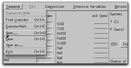
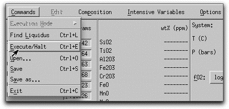
For this sample problem, you will use a saved bulk composition. Open an Xwin terminal, navigate to the directory where you have previously stored the MELTS software, and open the program. Once the graphical interface has opened, click Commands &rarr Open... to select from previously saved compositions.
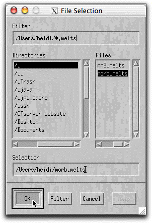
Select the morb.melts file you used in Sample Problem 1 and click Ok. If you do not have a file named morb.melts, follow the directions below to create one.
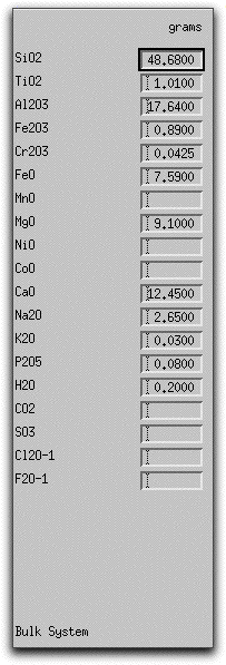
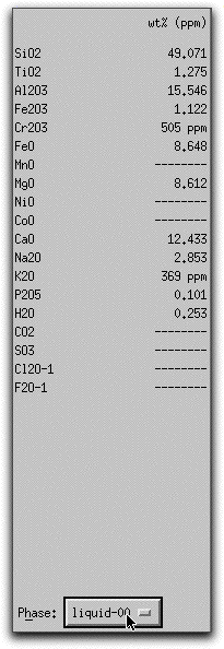
The morb.melts composition should have the following weight percent oxide values listed in the Bulk System Panel:
If you need to create a morb.melts file, type the values above into the boxes corresponding to the major oxides and volatile constituents. Then click Commands &rarr Save As... to open the Save As menu.
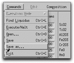
Name this composition "morb.melts" and click the Ok button. Do not forget the .melts extension or you will not be able to locate the file with the Open command in the future.
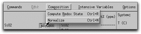
Note that morb.melts contains 100.36 grams of oxide components in the liquid. For practice, normalize the composition before continuing to construct the model. Click Composition &rarr Normalize and check that the total mass of the liquid changes to 100.00 grams in the System Display Panel.
TEMPERATURE AND PRESSURE
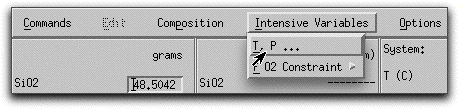
Before you assimilate any material into this composition, allow it to crystallize a bit under isothermic, isobaric conditions. From Sample Problem 1, you know that the predicted liquidus temperature of the morb.melts composition at 1000 bars is 1229.1° C. By starting the model at approximately these conditions, you know the composition will begin as a single liquid phase and immediately precipitate solids when the temperature drops below 1229°. Click Intensive Variables &rarr T, P...
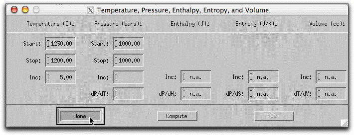
and change the starting and stopping temperatures to 1230° and 1200° C, respectively. Make sure the temperature increment is set to 5.00 so that the calculation generates enough data points to make a graph later.
CHOICE OF THERMODYNAMIC POTENTIAL AND THE OTHER THREE CONSTRAINTS
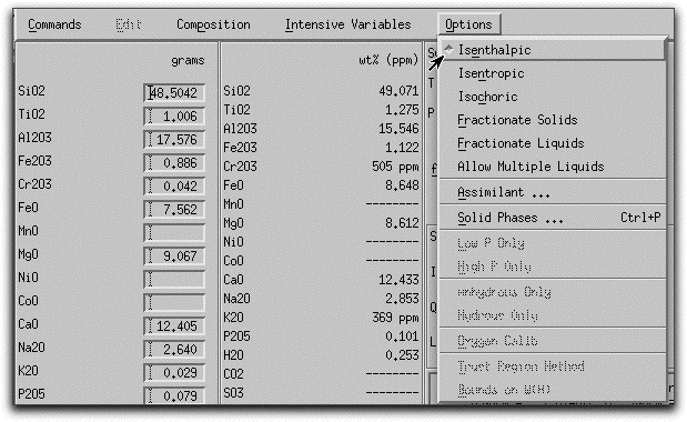
From Sample Problem 1, you know that MELTS minimizes the Gibbs free energy by default, and that you must activate alternative thermodynamic potentials in the Options menu. Minimizing the Gibbs free energy requires the temperature and pressure to remain constant at each step along the calculation path, which is what we want in this case, so there is no need to change the thermodynamic potential. Similarly, the oxygen fugacity constraint in the morb.melts file is already set to "absent," which means the system will evolve without an oxygen buffer. MELTS also calculates a closed-system, equilibrium path by default, so there is no need to inspect these menus.
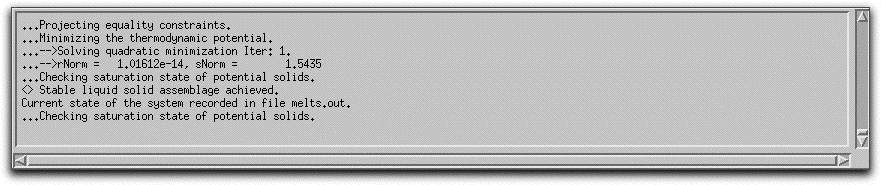
Click Commands &rarr Execute/Halt to begin the calculation.
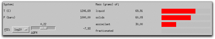
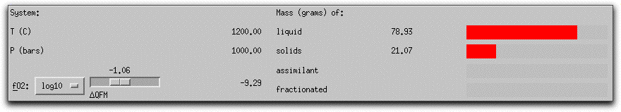
MELTS completes this portion of the calculation in six five-degree steps. When it has found the equilibrium assemblage at the final step, there are 21.07 grams of solid phases, as shown in the System Display Panel.
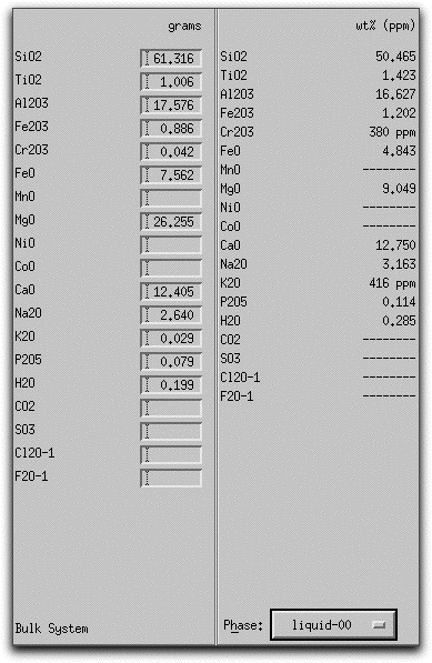
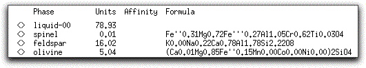
The solids consist of spinel, feldspar, and olivine. Their stoichiometric compositions are listed in the Phase Display Panel.
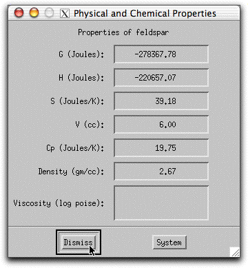
Double click on any phase listed in the Phase Display Panel to bring up the Physical and Chemical Properties screen.
Click on the button in the Phase Composition Panel and select "liquid" to display the weight % oxides of the liquid.
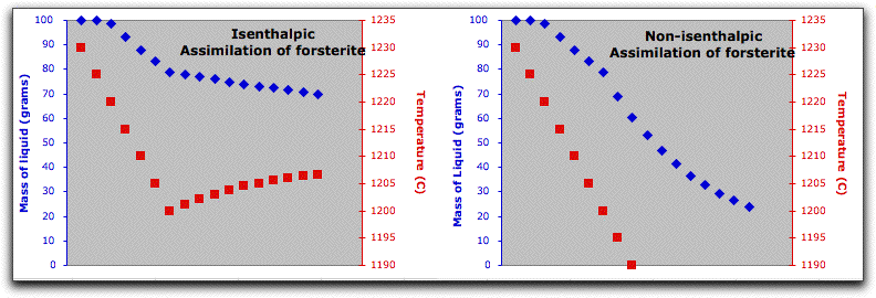
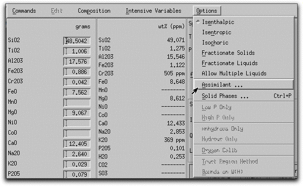
Now that some solids exist, use MELTS to predict the thermodynamic consequences of assimilating a large block of cold, solid material under isenthalpic conditions. Click Option &rarr Isenthalpic to minimize the enthalpy of the system instead of the Gibbs free energy.
Next, click Intensive Variables &rarr T, P... to open the temperature and pressure menu. Because the calculation will conserve enthalpy while it assimilates a substance with a drastically different temperature and chemical composition, MELTS will need to allow the temperature to vary. By giving MELTS a temperature to stop at, you can tell it how long to run the calculation. Set the stopping temperature to 1100°. Do not set an increment for temperature. Leave the pressure settings at 1000 bars.
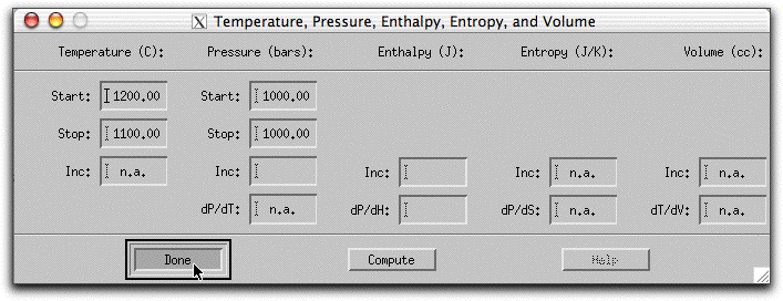
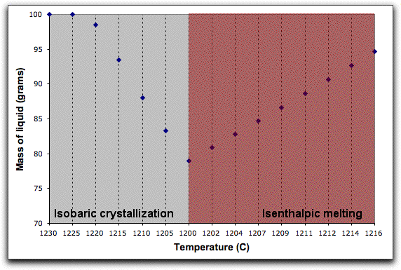
A word about the Enthalpy boxes. Entries in the Inc field either add or subtract enthalpy from the system in addition to the enthalpy that the system acquires from the assimilant in units of Joules. So, for example, if you set the Enthalpy Inc field to 1000 Joules, MELTS will add 1000 Joules of energy to the system enthalpy, then hold it steady at that amount and recalculate the equilibrium phases and required temperature at that enthalpy. This is illustrated in the figure below, which shows the system temperature increasing and the solid phases melting in response to these conditions.
The dP/dH button does something else.
We donÕt want to do any of these things. Instead, we want the only enthalpy to come from the assimilant. So leave the temperature, pressure menu as below:
Next, you need to characterize the assimilant. Click Options &rarr Assimilant... to open the Assimilant menu.
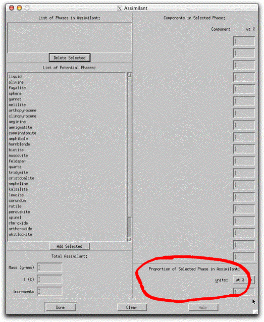
The Assimilant menu should look like this. Pay close attention to the bottom right-hand side of the screen, which must be visible in order to make the assimilation model work. If you cannot see this portion of the menu, enlarge the menu using the tool in the lower right hand side of the screen.
Double click "olivine" in the List of Potential Phases box. The name of this phase is added to the List of Phases in Assimilant box.
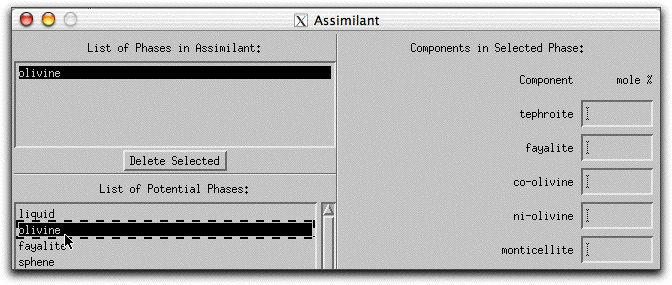
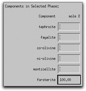
Now characterize the composition of the olivine in mole% components on the right hand side of the Assimilant menu. Set the composition to be 100% forsterite by typing "100.00" into the forsterite box.
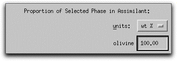
Because MELTS can calculate assimilants that contain more than one mineral phase, you must tell the program the relative proportion of each phase. For this sample calculation, the assimilant should be entirely forsterite. Type 100.00 into the box in the lowest right-hand corner of the Assimilant screen. The units: button above the box can be used to enter either wt% or volume%.
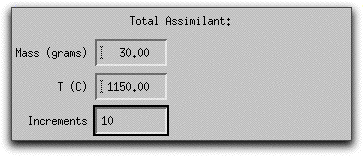
Next you need to tell MELTS how much of the assimilant, which is now defined as 100% forsteritc olivine, to add.