Sample Problem 1: Crystallizing MORB
The purpose of this first sample problem is to introduce you to the MELTS interface by describing the setup for modeling crystallization of a theoretical MORB liquid. After working through this sample problem, you will (1) understand which system parameters you can change and the general order in which you should change them before beginning MELTS modeling; (2) recognize the locations of menus and buttons used to change and monitor these parameters; (3) know where and how MELTS displays results; and (4) understand how to save and retrieve output files.
This example assumes that you are working with the Mac OS X standalone version of MELTS.
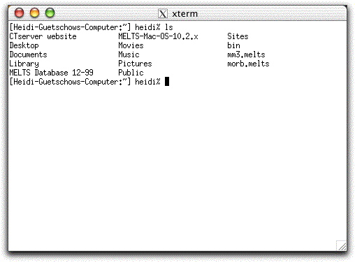
Open Xwin and navigate to the directory where you have saved MELTS. If you are unsure, use the unix command "ls" to list the files in the current directory.
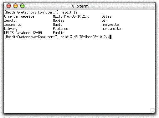
At the % prompt, type MELTS-Mac-OS-10.2.x or the appropriate file name.
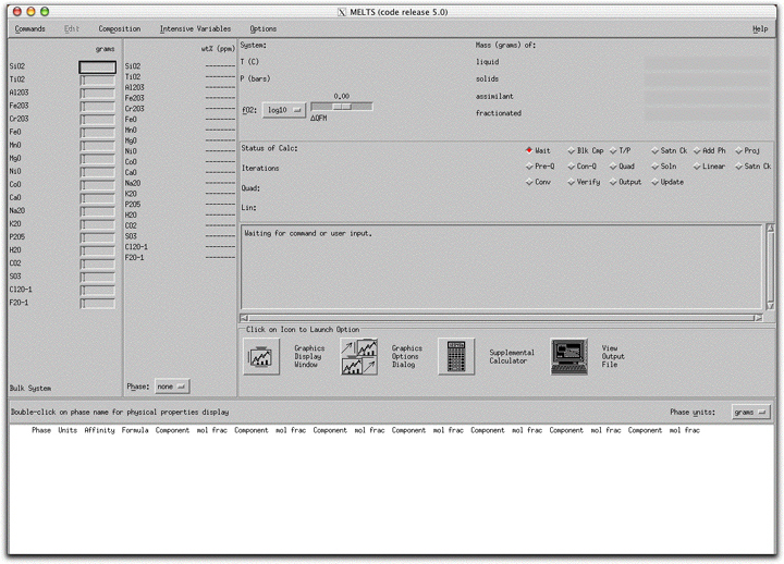
Answer "n" to the question that follows to open the MELTS interface
Six general system constraints require your attention before beginning a MELTS calculation:
The proceeding pages walk you through the menus that control these constraints, point out display features of the MELTS interface, and briefly discuss this first calculation.
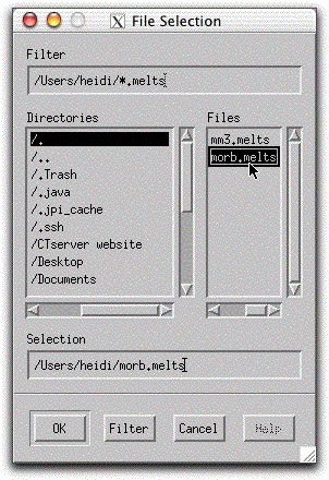
Load a previously saved bulk composition and set of system parameters by clicking Commands → Open...
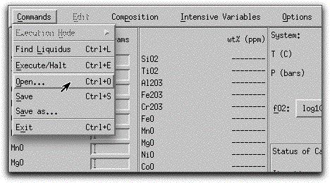
and selecting the file morb.melts.
If you have downloaded the morb.melts file, you should use it in this example. The morb.melts composition should have the following oxide values listed on the Bulk System Display Panel:
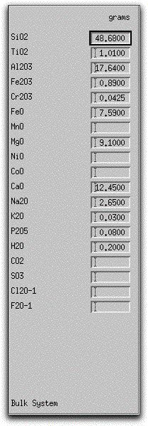
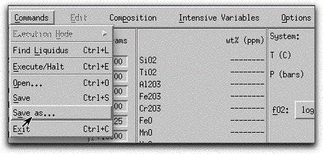
If you have not downloaded morb.melts, click on the box next to each oxide and enter the values above by hand. Next, save this composition with the name morb.melts by clicking Commands → Save as... Be sure to replicate the settings described in the rest of this sample so that you can follow along.
The Bulk System Display Panel displays the bulk composition of the system on the far left-hand side of the screen. MELTS displays oxides and common volatile components in grams. The morb.melts file contains 100.36 grams of oxides. Because MELTS is calibrated on natural rock compositions, as opposed to synthetic or theoretical compositions, it is important to begin calculations with bulk compositions that resemble natural systems. This means that under most circumstances, your MELTS model should begin with a bulk composition containing at least SiO2, TiO2, Al2O3, Fe2O3, FeO, MgO, CaO, Na2O, and K2O. If you omit from the bulk composition an oxide that plays a pivotal role in the chemical evolution of the magma, such as Note that the MELTS database currently does not contain sufficient data to model Cl and F behavior, but it does contain data on magmatic H2O, CO2, and SO3 that enable it to model these species.
Regardless of the precision of entered oxide values, MELTS maintains an internal precision of +/- 0.01 grams. MELTS normalizes the bulk composition to 100.00 grams at the beginning of each calculation. Normalize the morb.melts composition manually by clicking Composition → Normalize.
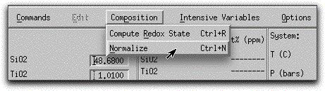
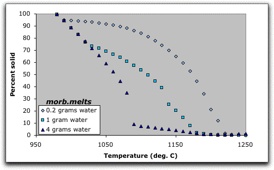
Normalizing compositions that do not total 100.00 grams provides an easy way to study the effect of critical oxides or volatile components in a single bulk composition. For example, if you would like to know how the concentration of water affects the crystallization sequence of the morb.melts model, subtract or add H2O to the bulk composition, normalize it, and allow it to cool to 980 °C. Repeating the crystallization sequence with increasing amounts of water reveals the acceleration of crystallization due solely to greater water content, as shown in the figure below.
ADDITIONAL COMPOSITION DISPLAY PANELS
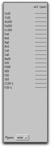
Next to the Bulk System Display Panel is the Phase Composition Display Panel. Once you have initiated the system and MELTS has generated at least one phase, this panel shows phase composition in weight percent oxides. Click on the box at the bottom of the panel labeled "Phase: none" to select the phase to display. This panel updates at each step along the calculation path, so the composition displayed is essentially an instantaneous composition of the phase as it is generated. Because the liquid is treated as a single phase in MELTS calculations, it can be displayed in the Phase Composition Display Panel. Try displaying the liquid phase here during the morb.melts calculation and watch its composition evolve as various phases approach the liquidus.
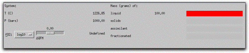
At the upper right-hand side of the screen, MELTS displays the masses of the liquid and cumulative solids in the system in the Liquid/Solid Display Panel. At any time during a calculation, you can quickly ascertain the total mass of liquid and solid components within the system by looking at the numbers next to the red bar graphs in this panel. The sum of these numbers always equals the total number of grams of material in the system. All saved compositions, such as morb.melts, display as entirely liquid in this panel before they have been equilibrated.
Two additional bar graphs labeled "assimilant" and "fractionated" represent quantities of material that have either been added to or extracted from the initial bulk system composition. These are useful in more complicated calculations when it is important to monitor the amounts of these external components and observe the timing of changes to the system of liquid + solid with the addition of assimilant material or the removal of fractionated material. In an assimilation model, the "assimilant" bar graph refers to the cumulative material that has been added to the system, and it fills progressively as more material is added.
In a fractionation model, the "fractionated" bar graph refers to the cumulative amount of fractionated liquids or solids, while the "solids" bar graph refers to the amount of solids generated in a given step. Newly generated solids are immediately added to the cumulative "fractionated" material before data is written to the output file.
INTENSIVE VARIABLES: T, P REACTION PATHS AND OXYGEN FUGACITY
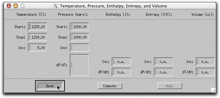
Clicking on the Intensive Variables button on the top of the MELTS interface allows you to set the temperature, pressure, entropy, enthalpy, volume, and oxygen fugacity variables that affect the calculation independent of the amount of material present in the system. The previously saved morb.melts file specifies a temperature and pressure path along which MELTS will calculate equilibrium liquid and solid compositions. Click Intensive Parameters → T,P... to review the temperature and pressure settings.
According to this temperature-pressure path, MELTS will begin the calculation at 1500° C and work its way down to 980° C in five-degree increments. If you do not specify an increment, MELTS will traverse the temperature-pressure path in one large step, obscuring intermediate crystallization events. If you specify a very small interval, the calculation will take longer and the output files will be larger. However, if your computer is relatively fast, you may wish to effectively slow down the calculation by specifying very small temperature or pressure steps.
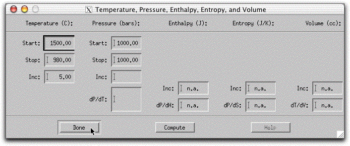
Because the pressure in morb.melts is set to 1000 bars in both the Start and Stop boxes, the calculation will be isobaric. To simulate a non-isobaric system, specify both a beginning and ending pressure and an increment of change in the T, P... menu. Alternately, you can set MELTS to follow a dP/dT path, and the program will calculate the required increment and final pressure. A sample non-isobaric problem is provided in the next section. A calculation path that specifies both temperature and the pressure change over different numbers of steps, causes MELTS to take the larger number of steps.
MELTS must have starting values for both temperature and pressure before it begins a calculation. If one of these variables has not been specified, an error message will appear when you try to run the model.
CHOICE OF THERMODYNAMIC POTENTIAL
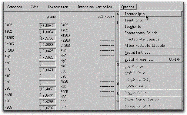
By default, MELTS minimizes the Gibbs free energy of the system by holding temperature and pressure constant at each step along a specified temperature-pressure path. In certain circumstances, it is preferable for MELTS to minimize a different thermodynamic potential such as the enthalpy or entropy. Minimizing one of these alternative potentials is more complicated numerically, and requires either the temperature or the pressure to vary. When this is the case, MELTS must follow a different calculation path. For example, to model isenthalpic processes, MELTS holds the pressure and the enthalpy constant and allows the temperature to vary at each step along the calculation path. For this reason, input boxes for Enthalpy, Entropy, and Volume gradients are positioned next to the Temperature and Pressure input boxes. In order to enter values into these boxes, click on Options button and select from the menu of isenthalpic, isentropic, isochoric constraints. For this sample problem, leave the system in its default state.
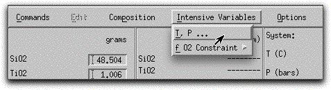
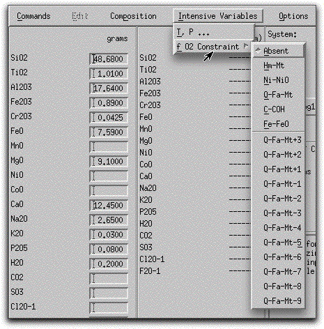
The final intensive variable to set before beginning a MELTS calculation is the oxygen fugacity of the system. By clicking Intensive Variables → f O2 Constraint and selecting from among the listed options, you may impose an oxygen fugacity buffer on your MELTS model or leave it in its default mode, absent. MELTS can calculate along the reference oxygen fugacity buffers hematite-magnetite (HM), nickel-nickel oxide (NNO), quartz-fayalite-magnetite (QFM), one or more logarithmic units above or below QFM, and iron-wustite (IW). For the purposes of this sample problem, do not impose an oxygen fugacity on the system.
Caution is advised should you choose to impose an oxygen fugacity constraint - although it is appropriate for short portions of some magmatic reaction paths, in most cases it is unrealistic to model an entire crystallization sequence along an oxygen-buffered path. Few experimental data have been collected under oxygen-buffered conditions, and it is difficult to imagine a magmatic source region on Earth where such a buffer could be continuously present.
Iron partitioning strongly affects both mineral compositions and crystallization sequences because the formation of some minerals preferentially removes ferric iron from the bulk liquid to fill crystallographic sites, thus indirectly setting the oxygen fugacity of the magma on the liquidus. If no ferric iron is available in the melt, these sites are filled with other oxides (such as TiO2) and the system moves towards a more O2-rich state. The bulk ferric/ferrous iron ratio of the system must be entered or calculated for MELTS to simulate iron partitioning. In the case of morb.melts, the ferric/ferrous ratio of the system has been set by entering Fe2O3/FeO analyses of MORB glass. MELTS can also compute the appropriate Fe2O3/FeO ratio based on temperature, pressure, and oxygen fugacity constraints. In the next sample problem you will learn how to calculate an Fe2O3/FeO ratio for your own bulk composition.
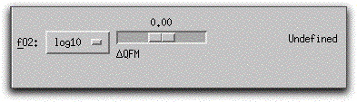
Oxygen fugacity conditions are displayed on the System Display Panel, where undefined indicates that no constraint has been set. Once MELTS has begun a calculation, it displays the oxygen fugacity of the system relative to the QFM buffer above the delta QFM bar and in base 10 logarithm units to the right of the bar. To display the fugacity relative to a different buffer, click on the button to the left of this bar labeled "fO2: log10" and select a reference buffer. The value displayed to the right of the delta QFM bar changes to display the difference between the system oxygen fugacity and the selected buffer.
SPECIFYING OPEN OR CLOSED SYSTEM BEHAVIOR
By default, MELTS assumes the system is closed to mass transfer and performs equilibrium crystallization calculations. The morb.melts file has been left in this default mode. Click the Options menu button to confirm that the Fractionate Solids, Fractionate Liquids, and Assimilant options have not been invoked. Fractionation and assimilation models will be discussed further in Section 22: Sample Problem 3.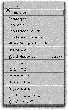
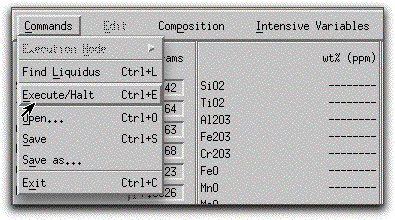
To begin a MELTS calculation, you can either click Commands → Execute/Halt to initialize the system and immediately begin down the temperature-pressure path specified in the Intensive Variables menu,
or click Commands → Find Liquidus to calculate the liquidus temperature.
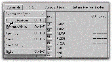
For beginning MELTS users, it is advisable to find the liquidus before beginning a calculation to ensure that the temperature specified in the Intensive Variables menu is appropriate. Find the liquidus of the morb.melts composition before continuing on to the next step.
Using the settings from the T, P... constraint panel as an initial guess, MELTS determines whether the composition is at its liquidus by searching for the presence of any equilirbrium solids. At 1500° C, MELTS finds no equilibrium solids in morb.melts, concludes that the composition is far above its liquidus temperature, and repeats the search at 1450° C. MELTS repeats this procedure at 50 degree intervals until it finds solids that are in equilibrium with the liquid, then iteratively raises the temperature again until the solids disappear. It follows this procedure, using successively smaller intervals until it finds the temperature just above phase saturation. This calculated liquidus temperature is assigned to the starting temperature of the system in the T, P... constraint panel.
MELTS exhibits its progress towards the liquidus on the status display screen in the center of the interface. This screen outputs brief descriptions of changes to intensive variables, the addition of new phases to the solid assemblage, the point at which the program achieves stable liquid/solid stability, and the number of iterations and type of equation it is working on. This information is also printed to the output file MELTS generates when it is properly exited. A scrollbar on the right-hand side of the output screen allows you to go back through this information without exiting.
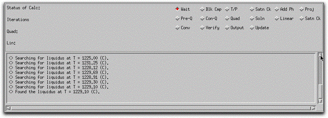
At this point you have loaded a saved composition, normalized it to 100.00 grams, and found its liquidus at 1229.10° C. It is a good idea to record the temperature and pressure of the system at this point, since small changes to the starting conditions sometimes have big effects on the results and you may want to run this model several times before opening the output files.
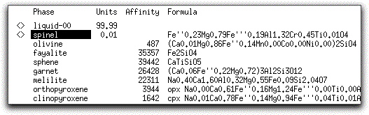
Before you allow this MORB to crystallize, examine the Phase Display Panel at the bottom of the screen. MELTS considers all 33 solid and liquid phases in its database as potential phases. MELTS finds the composition of each potential phase that is closest to equilibrium with the liquid and displays this composition next to a quantitative measure of its distance from equilibrium with that liquid, the Affinity. Phases that are about to become stable are those with an Affinity close to zero. At its liquidus, morb.melts has three phases with relatively small Affinity: spinel (-6), feldspar (349), and olivine (708). Use the scrollbar on the far right-hand side to locate all three phases. Because it has a negative affinity, spinel is in a supersaturated state. When a phase achieves equilibrium, and liquid or a solid mineral appears, the Affinity column is left blank and the phase name is marked with the <> symbol.
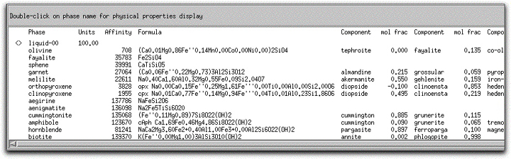
The chemical formula of each phase is displayed to the right of the Affinity column. These atomic formulae reflect atomic ordering of elements in different structural sites. MELTS refines the compositions of solid solution minerals once they stabilize on the liquidus and each time there is a change in intensive variables, and you can monitor the evolution of the entire assemblage during the calculation. To the right of the mineral formulae, the corresponding molar fractions of their components are displayed. MELTS records only the component mole fraction data in the output files when you exit the program, but you can recalculate the formula data with the Mineral Calculator, explained in a later section.
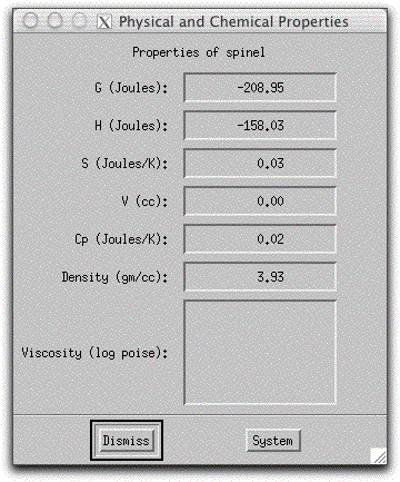
As a consequence of finding the liquidus, MELTS computes initial values for the enthalpy (H), entropy (S), and volume (V) of the liquid, which it uses for subsequent calculations. To view these values along with the Gibbs Free Energy (G), chemical potential (Cp), density, and viscosity, double-click the button labeled "liquid-00"
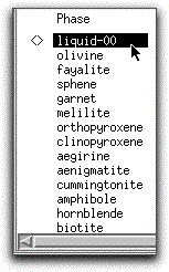
to open the Physical and Chemical Properties screen.
Note that you can toggle this screen to display either the selected phase or the system properties using the button in the lower right-hand side of the screen.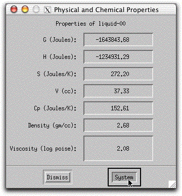
Now that you have been introduced to all of the display panels and confirmed that morb.melts' constraints are correctly set, it is time to run the crystallization model. The following section discusses the first four temperature steps in detail before discussing the final results and output files, so to follow along, click on Intensive Variables &rarr T,P... and change the Stopping temperature to 1224.10 degrees. Then click Commands &rarr Execute/Halt or control + e to begin the calculation.
Once you click Commands &rarr Execute, the Output Display Panel lists calculation progress and diamond-shaped indicator lights blink on and off as the program works on different aspects of the calculation. When the message, "<> Stable liquid solid assemblage achieved. Current state of the system recorded in file melts.out" appears, the calculation of the first five-degree step is complete and MELTS has generated data files for each stable phase. MELTS does not write the data to these files unless it is exited properly using Commands &rarr Exit, as shown at the end of this section.
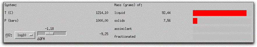
The current temperature, pressure, and oxygen fugacity of the system are displayed with the proportions of solid and liquid components in the System Display Panel. Note that there are now 0.01 grams of solids and 99.99 grams of liquid. The oxygen fugacity has decreased slightly from -1.21, -9.12 to -1.22, -9.18 base 10 logarithm units.
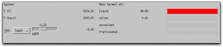
Because you performed a Find Liquidus command before beginning the calculation, the system started at its liquidus, and solids formed after this first five-degree temperature decrement. In the Phase Display Panel, MELTS identifies the 0.01 grams of solid material indicated in the System Display Panel as the phase spinel. The <> symbol indicates spinel is in equilibrium with the liquid and the chemical formula and component mole fractions are displayed to the right.
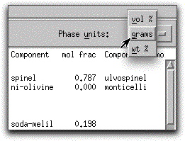
The Units column in the Phase Display Panel displays grams by default. However, you can change the Units column to display weight percent (wt%) or volume percent (vol%) using the button in the upper right-hand corner of the panel.
Open the Physical and Chemical Properties screen for the newly-precipitated spinel by double-clicking on its name in the Phase Display Panel. Compare its density (3.93 g/cc) to that of the liquid (2.68 g/cc) Ð as the calculation progresses, it is important to keep in mind the physical nature of the model.
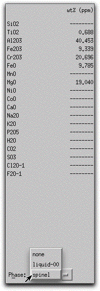
Now that more than one phase is present, you can activate the Phase Composition Display Panel. Click on the button at the bottom of the panel labeled Phase: and select spinel to view the chemical composition of the spinel that formed during this step of the calculation in weight percent oxides.
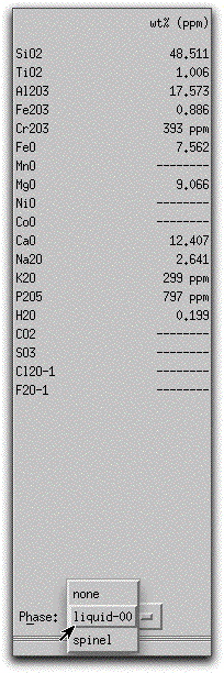
Click on the button again and select liquid-00. The composition of the remaining 99.99 grams of liquid is not very different from the bulk composition displayed to the left in the Bulk System Display Panel because a very small amount of solids has formed. For the rest of the calculation, keep liquid-00 active in this panel and watch it change as significant amount of minerals crystallize and remove chemical constituents from the liquid.
Click on Intensive Variables &rarr T, P... and change the stopping temperature to 1219.30.
At 1219.10° C, 0.02 grams of spinel and 1.84 grams of feldspar are in equilibrium with the liquid.
Examine the Phase Display Panel again. From the chemical formula and fractional components of the feldspar, you can see it has a high anorthite content.
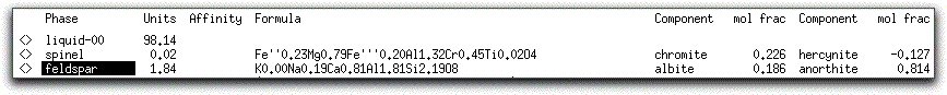
It is important to reiterate that, although the grams of stable phases in the Phase Display Panel are cumulative, the compositions reported there are instantaneous and they evolve as proportions of oxides in the liquid change. For example, the 0.02 grams of spinel listed at this step is the sum of the 0.01 grams that crystallized at 1224.10° C, plus 0.01 new grams that crystallized at 1219.10° C.
Click Intensive Variables &rarr T, P... and change the stopping temperature to 1214.10°.
At 1214.10° C, spinel remains a very minor phase with only 0.02 grams present, while the amount of solid feldspar in the system has increased to 6.08 grams, and 1.47 grams of forsteritic olivine have joined the assemblage.
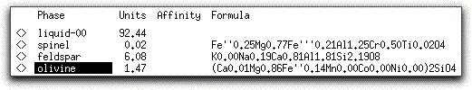
The System Display Panel shows that 7.56 grams of solid phases have crystallized from the liquid by the time it has cooled 15° C from its liquidus. Double-clicking on each phase in the Phase Display Panel reveals that the calculated density of each solid phase except for feldspar is greater than that of the liquid.
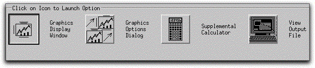
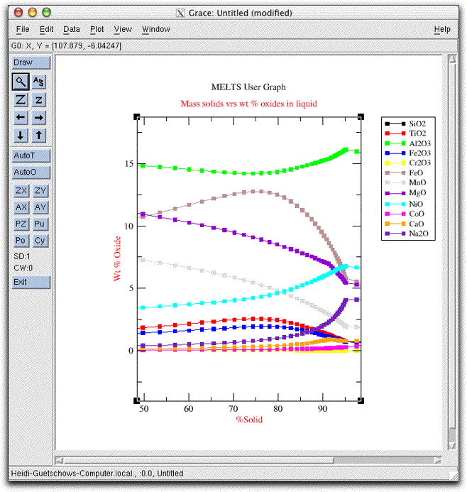
If you downloaded the Grace program as outlined on the downloads page, you can view a graph of the chemical evolution of the morb.melts liquid by clicking the furthest-left button on the Graphics Options Panel labeled Graphics Display Window.
Drag the graphics window, called Grace: Untitled (modified), off to one side of the screen so that you can find it easily. Next, set the calculation to run until the assemblage is completely solid by clicking Intensive Variables &rarr T, P... and changing the stopping temperature to 975.00°. Then click Commands &rarr Execute to allow the calculation to continue along the temperature-pressure path you just set. Click on the Grace graphics window again to watch graphical output of the calculation.
Since the temperature decrement is five degrees and the system was at 1214.10° C, the closest it comes to 975° is 979.10. By this temperature the system has completely crystallized, and three additional phases have come on the liquidus: clinopyroxene, apatite, and water. The final composition of the liquid is listed as a potential phase in the Phase Display Panel.
Examine the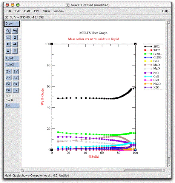
Click Commands &rarr Exit to close MELTS and save the data to output files.
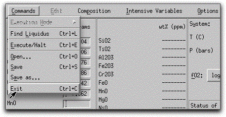
Composition and physical data about each phase formed during the calculation has now been saved in a separate file with a .tbl extension: melts-liquid.tbl, spinel.tbl, feldspar.tbl, olivine.tbl, clinopyroxene.tbl, apatite.tbl, and water.tbl. These files are useful for interpreting the evolution of each phase over the course of the calculation, but not useful for interpreting interaction between phases or changes to the systemÕs intensive variables. A separate file called melts.out contains the phase data organized by each progressive step in the calculation and is helpful for interpreting the behavior of the system as a whole.
Each time you exit the program using Commands &rarr Exit, MELTS automatically saves these .tbl and .out files. MELTS overwrites previously-existing files without warning, so it is imperative that you rename data files immediately if you wish to examine them later.
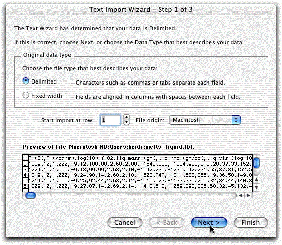
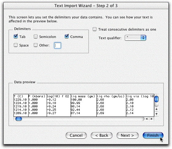
The data in the.tbl files are delimited differently from the data in the .out files. To manipulate the data in a spreadsheet program, you must tell the program how to divide it into columns. To open the melts-liquid.tbl file in MS Excel, for example, click File &rarr Open, followed by Show: All Documents. (All .tbl and .out files will still look grey and "unclickable".) Double-click on melts-liquid.tbl.

On the next screen, click Delimited.
On the next screen, highlight Comma, then click Finished.
Now the screen should look like this:
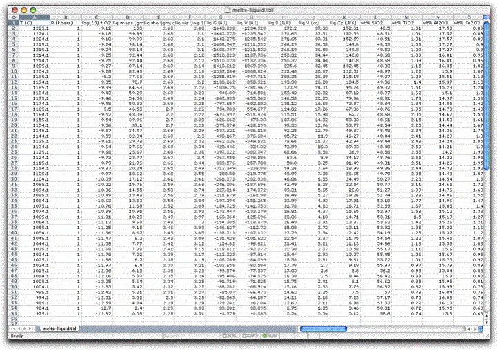
Note there are two identical rows of data for temperatures 1224.1, 1219.1, and 1214.1°. This is because MELTS records data every time it finds a stable solid/liquid assemblage, which it does at both the beginning and ending of each new temperature-pressure path. Thus in the first step of this calculation, MELTS saved data from the starting stable assemblage at 1229.3° and from the ending stable assemblage at 1224.3°. In the second step, it saved data from the starting assemblage at 1224.3° and from the ending stable assemblage at 1219.1°. And so on. It is a good idea to delete these duplicate data now to avoid confusion.
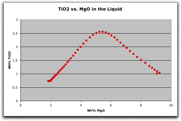
As you begin to interpret the results from your MELTS model, it is often instructive to simply plot the major oxides of the liquid versus a fractionation index, such as wt% MgO. In this case, you can see that something happens to the system at about 1129 degrees that dramatically changes the chemical evolution of the liquid.
To investigate this, you need to examine the melts.out file from this calculation. Click File &rarr Open, Show All Documents, and double-click on melts.out. The same delimited screen should open.
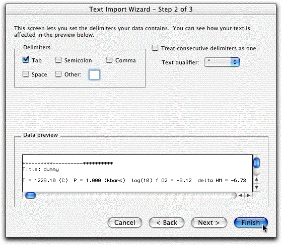
This time, however, click Delimitedand leave Tabs highlighted and click Finished.
The melts.out file should look like this:
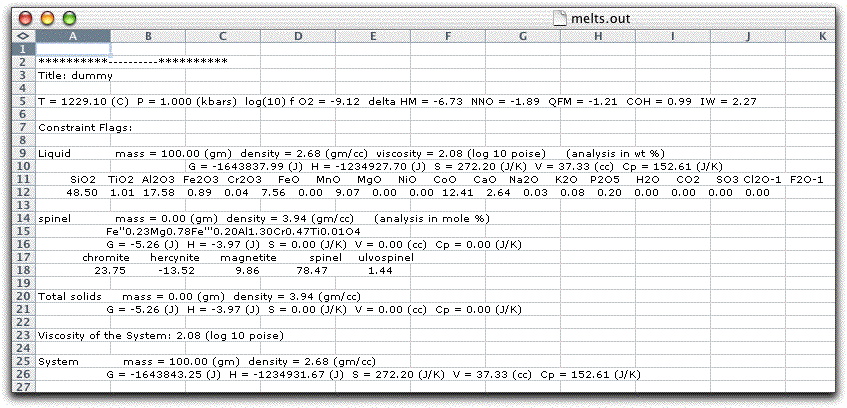
Make sure you can see all of the temperature, pressure, and oxygen fugacity output listed in row five to prevent overlooking important data. If you can't see all of row five, something went wrong on the Text Import Wizard screen. Close it without saving and try again.
All of the constraints and phase data from each step of the calculation are recorded in the melts.out file: the system T, P, fO2, etc., as well as the names, compositions, and physical characteristics of each phase stable during that step.
Scroll down to 1124.10° C. No new phase appears during this step, so the change in the chemical composition of the liquid must result from a compositional change of one of the existing phases. Compare the compositions of olivine, clinopyroxene, feldspar, and spinel at 1124.10° C and one step earlier, at 1129.10° C.
The composition of spinel has become significantly more Fe2+- and Ti-rich and Al-poor over this single temperature interval, and continues to evolve this way until the system is entirely solid. There is no major change in any of the other minerals during this interval. Thus, it is likely that the changing composition of spinel caused the change in the chemical evolution of the liquid. There are many other interesting changes in both the chemical and physical